第 5 章 密度图

5.1 基本密度图

data <- read.table("Datas/1_OneNum.csv", header=TRUE)

# Make the histogram
data %>%
  filter( price<300 ) %>%
  ggplot( aes(x=price)) +
    geom_density(fill="#69b3a2", color="#e9ecef", alpha=0.8)

5.1.1 自定义样式

data %>%
  filter( price<300 ) %>%
  ggplot( aes(x=price)) +
    geom_density(fill="#69b3a2", color="#e9ecef", alpha=0.8) +
    ggtitle("Night price distribution of Airbnb appartements") +
    theme_ipsum()

5.2 镜像密度图

data <- data.frame(
  var1 = rnorm(1000),
  var2 = rnorm(1000, mean=2)
)

# Chart
ggplot(data, aes(x=x) ) +
  # Top
  geom_density( aes(x = var1, y = ..density..), fill="#69b3a2" ) +
  geom_label( aes(x=4.5, y=0.25, label="variable1"), color="#69b3a2") +
  # Bottom
  geom_density( aes(x = var2, y = -..density..), fill= "#404080") +
  geom_label( aes(x=4.5, y=-0.25, label="variable2"), color="#404080") +
  theme_ipsum() +
  xlab("value of x")

5.3 分组密度图

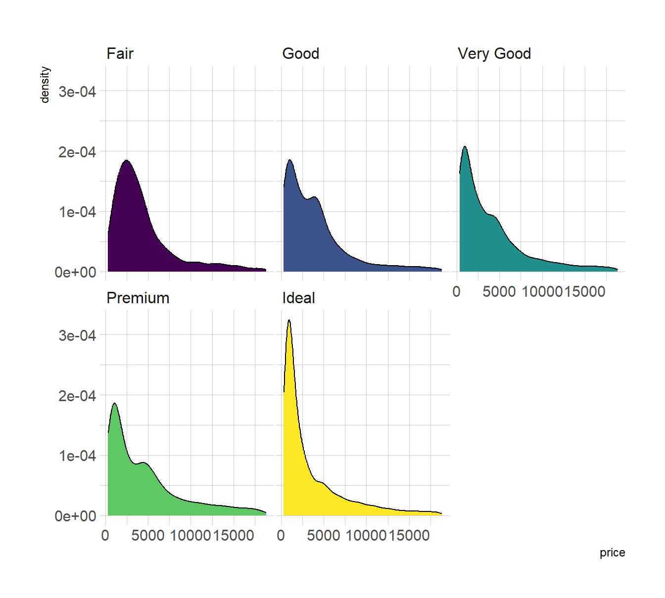
# The diamonds dataset is natively available with R.

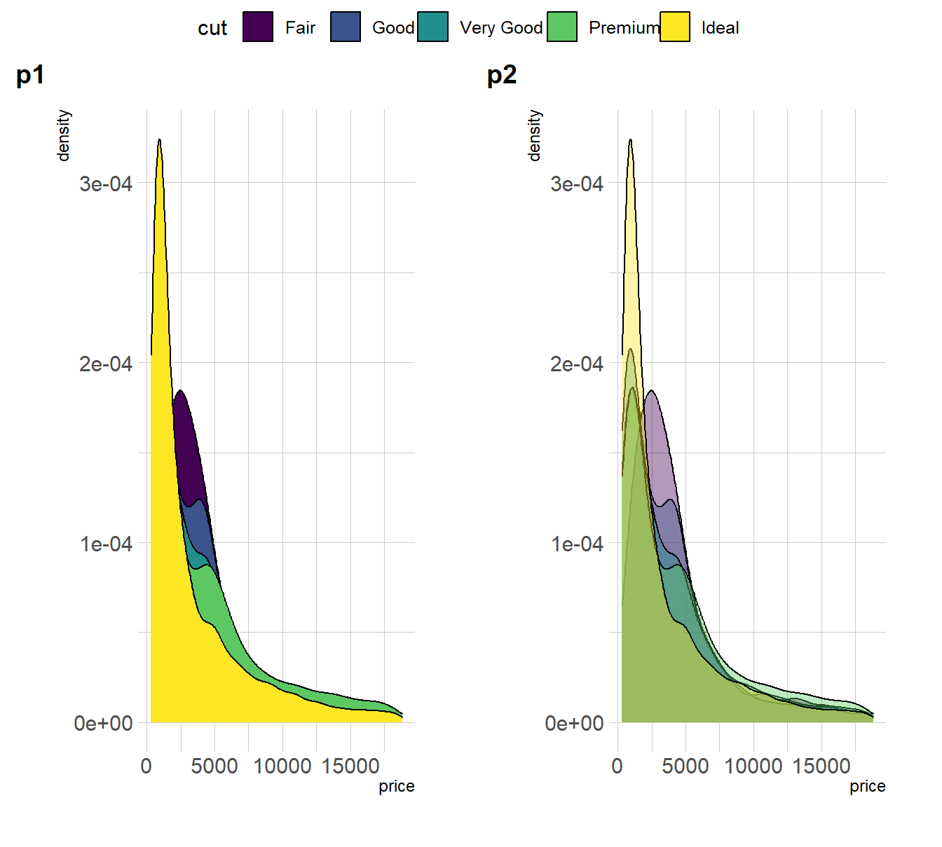
# Without transparency (left)
p1 <- ggplot(data=diamonds, aes(x=price, group=cut, fill=cut)) +
    geom_density(adjust=1.5) +
    theme_ipsum()


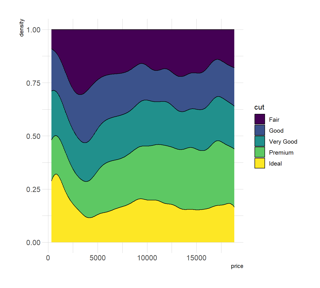
# With transparency (right)
p2 <- ggplot(data=diamonds, aes(x=price, group=cut, fill=cut)) +
    geom_density(adjust=1.5, alpha=.4) +
    theme_ipsum()
ggarrange(p1,p2,labels = c("p1","p2"),common.legend = T)

data <- read.table("Datas/probly.csv", header=TRUE, sep=",")
data <- data %>%
  gather(key="text", value="value") %>%
  mutate(text = gsub("\\.", " ",text)) %>%
  mutate(value = round(as.numeric(value),0))

# A dataframe for annotations
annot <- data.frame(
  text = c("Almost No Chance", "About Even", "Probable", "Almost Certainly"),
  x = c(5, 53, 65, 79),
  y = c(0.15, 0.4, 0.06, 0.1)
)

# Plot
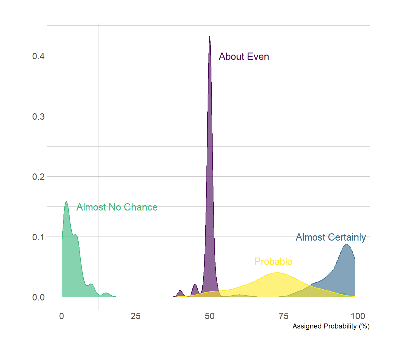
data %>%
  filter(text %in% c("Almost No Chance", "About Even", "Probable", "Almost Certainly")) %>%
  ggplot( aes(x=value, color=text, fill=text)) +
    geom_density(alpha=0.6) +
    scale_fill_viridis(discrete=TRUE) +
    scale_color_viridis(discrete=TRUE) +
    geom_text( data=annot, aes(x=x, y=y, label=text, color=text), hjust=0, size=4.5) +
    theme_ipsum() +
    theme(
      legend.position="none"
    ) +
    ylab("") +
    xlab("Assigned Probability (%)")

5.4 分面密度图

ggplot(data=diamonds, aes(x=price, group=cut, fill=cut)) +
    geom_density(adjust=1.5) +
    theme_ipsum() +
    facet_wrap(~cut) +
    theme(
      legend.position="none",
      panel.spacing = unit(0.1, "lines"),
      axis.ticks.x=element_blank()
    )

5.5 堆积密度图

 ggplot(data=diamonds, aes(x=price, group=cut, fill=cut)) +
    geom_density(adjust=1.5, position="fill") +
    theme_ipsum()